1 Lets have a look at dplyr.

dplyr is a grammar of data manipulation, providing a consistent set of verbs that help you solve the most common data manipulation challenges:

filter() picks cases based on their values.
arrange() changes the ordering of the rows.
select() picks variables based on their names.
mutate() adds new variables that are functions of existing variables
summarise() reduces multiple values down to a single summary.

These all combine naturally with group_by() which allows you to perform any operation “by group”.

All verbs work similarly:

The first argument is a data frame.
The subsequent arguments describe what to do with the data frame, using the variable names (without quotes).
The result is a new data frame.

Together these properties make it easy to chain together multiple simple steps to achieve a complex result. Let’s dive in and see how these verbs work.

1.1 first install dplyr and call the library:

install.packages("dplyr")

## Updating HTML index of packages in '.Library'

## Making 'packages.html' ... done

library("dplyr")

## 
## Attaching package: 'dplyr'
## 
## The following objects are masked from 'package:stats':
## 
##     filter, lag
## 
## The following objects are masked from 'package:base':
## 
##     intersect, setdiff, setequal, union

We can call head to see the first 10 rows of a dataset. I am using an available dataset which can be found on the dplyr library

starwars

head(starwars)

What does it have starwars? we can call column names function:

colnames(starwars)

##  [1] "name"       "height"     "mass"       "hair_color" "skin_color"
##  [6] "eye_color"  "birth_year" "sex"        "gender"     "homeworld" 
## [11] "species"    "films"      "vehicles"   "starships"

Now we can do some filtering with dplyr commands

humans <- starwars %>%
  filter(species == "Human")

humans_selected_columns <- humans %>% 
  select(birth_year, gender, mass, height, homeworld)

humans_bmi <- humans_selected_columns %>%
  mutate(bmi = mass / ((height / 100)  ^ 2)) %>%
  arrange(bmi, height, desc(birth_year)) %>%
  na.omit

We can visualize as many rows as we want

head(humans_bmi, 15)

Lets see if there is any relation between planet and bmi For that why dont we start with one plot? As before we start by installing the library and calling it:

install.packages("ggplot2")

## Updating HTML index of packages in '.Library'

## Making 'packages.html' ... done

library("ggplot2")

Lets try a boxplot

p <- ggplot(humans_bmi, aes(x=homeworld, y=bmi))

p <- p + geom_boxplot() 
p + geom_jitter(shape=16, position=position_jitter(0.2))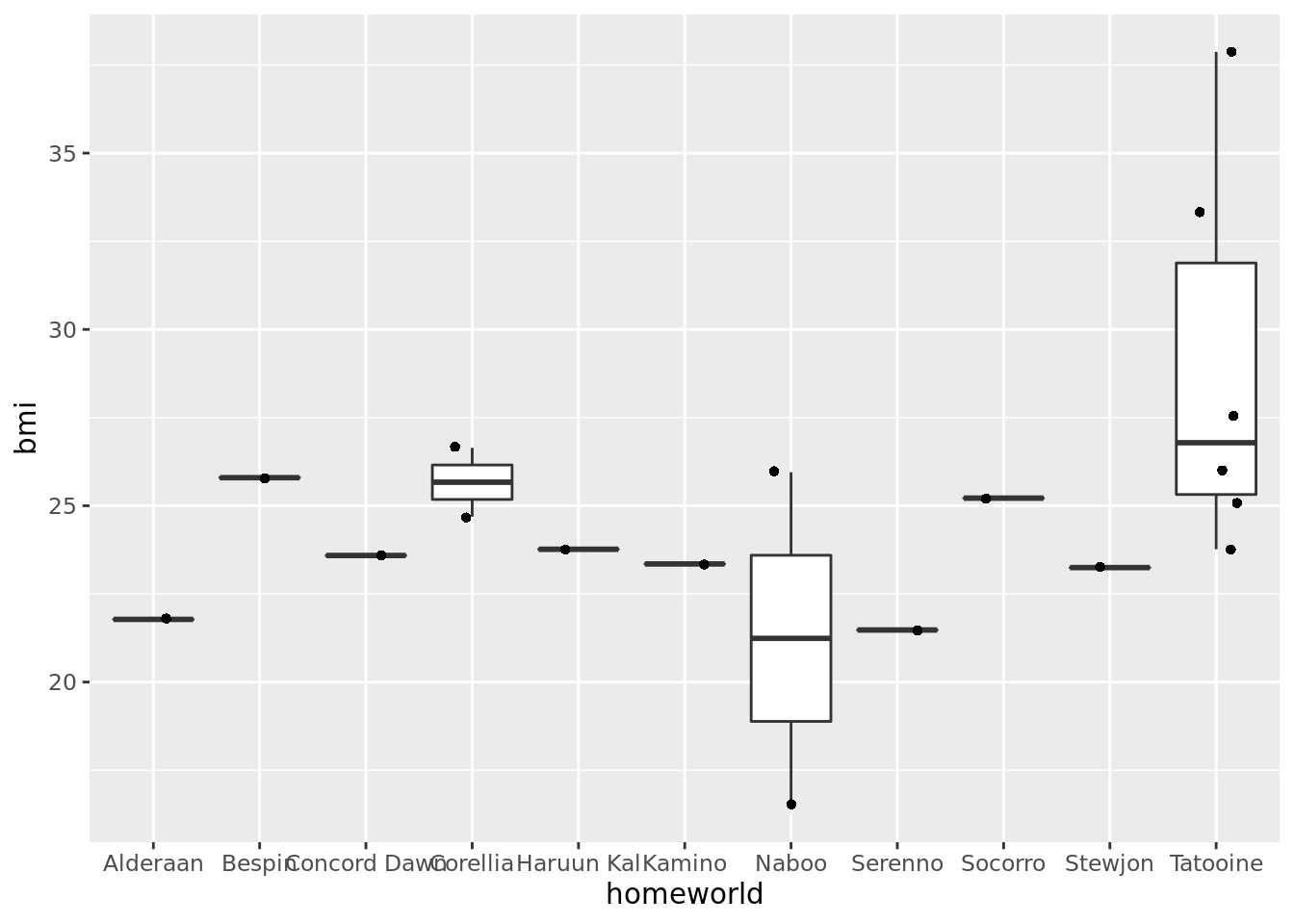

Apparently, Tattoine has a higher bmi than Naboo… but what if we have a statistic to test for it? The issue is that we have a low number of individuals (<10) and special statistics are needed.

Lets get those that have more than one human

humans_bmi %>% count(homeworld)

humans_filtered <- humans_bmi %>%
  filter(homeworld==c("Tatooine"))

head(humans_filtered, 10)